Physics-Based Simulation (BBP)

What BBP Adds

A physics-based simulated seismogram is computed from a rupture model propagating through a regional crustal velocity model. That is a different kind of object from an empirical estimate fitted to a single peak-acceleration number: it has a time base, a frequency content and a duration, so it can be compared with a real recording trace for trace rather than only at its peak. The heavy Fortran computation runs on an on-demand cloud instance that is started for the job and terminates when it finishes — not on the web server answering this page.

Building the Rupture (src) From ShakeMap Event Parameters

The pipeline builds a BBP scenario job (a "src" rupture description) directly from the USGS event parameters used everywhere else on this site:

• Fault geometry from the USGS moment tensor's first nodal plane (strike, dip, rake); when no moment tensor is published, a regional strike-slip default is used
• Fault dimensions from Wells & Coppersmith (1994) magnitude scaling, with the hypocenter centered down-dip at the USGS depth
• Method: Graves & Pitarka (GP), a hybrid broadband approach combining deterministic low-frequency wave propagation with a stochastic high-frequency component
• Rupture seed derived deterministically (via SHA-256, not Python's per-process-salted hash()) from the USGS event id, so re-running an event reproduces the same waveform across worker restarts

Selecting the 1D Velocity Model

A BBP velocity model is a layered one-dimensional crustal profile of seismic velocity and density, not a map — it can technically be applied anywhere, but it only physically describes the region it was built for. This service installs several California regional velocity-model packages and routes each earthquake to the model whose native extent contains its epicenter:

• LABasin500 (“SoCal” on the map) — Los Angeles basin / Southern California
• Mojave500 (“Mojave”) — the Ridgecrest & Mojave / eastern Southern California corridor
• CentralCal500 (“CenCoast”) — Coast Ranges, Central Valley, Parkfield
• NoCal500 (“NoCal”) — San Francisco Bay Area and northward
• SouthernSierra500-2 (“Southern Sierra Nevada”) — the Owens Valley / Lone Pine corridor

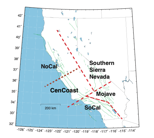
Every region shown above is installed in production. When an event's epicenter falls outside every native extent, the simulation runs against the geographically nearest installed region (an equirectangular distance to each region's extent) and the result is labeled an approximation — the map above shows which region that would be, even before it's picked. Location alone does not make an event ineligible: nothing in BBP validates that a rupture's tectonic style matches the crustal profile it runs against, so a Cascadia subduction-zone event, for example, is still simulated using a method built for shallow crustal ruptures, and that result is illustrative only. There are just two eligibility criteria: a magnitude of M5.0 or above, and at least one velocity-model region installed. Distance from a region's extent is not one of them — a Reno, Las Vegas, Portland or Mexicali earthquake is simulated against the nearest installed model and labeled an approximation, rather than being refused. An event below the magnitude floor is not simulated at all — see Standing Limitations for why that floor exists.

A separate 200 km limit does apply, but to a different distance: how far from the epicenter an individual site may be placed in the Simulation Lab, since that is the range over which the method is validated for a station. It constrains where you may ask for a seismogram; it has never governed whether the earthquake itself can be simulated.

Goodness-of-Fit: Scoring the Simulation Against Reality

A simulation that looks convincing in an animation is not necessarily accurate, so for each qualifying event this service measures the simulation against the real earthquake. It retrieves the recorded accelerations at seismic stations around the epicenter (via the same ObsPy/FDSN pipeline described in Observed Seismic Station Data — uncut acceleration, so nothing is trimmed before the comparison), submits them alongside a BBP simulation of the same event, and reads back the Broadband Platform's own goodness-of-fit residuals — the mean logarithmic bias between the observed and simulated response spectra.

The result is published as a goodness-of-fit report, shown on the event page under BBP Simulation Comparison with a full report page of its own and a downloadable PDF, with a verdict against a pre-declared pass band (a factor of two, i.e. a mean absolute bias of 0.69). Because a structure responds at its own period, the report states the bias period by period rather than as a single average and flags any period outside the band — a simulation can pass on the mean while being well off at a specific period.

Standing Limitations

• A simulation is not a site-specific engineering estimate. It describes what a modelled rupture would produce under a modelled crust. Use it to understand the character of shaking, not as a design value for a particular structure.
• The rupture is derived, not observed. Fault dimensions come from magnitude scaling, and the moment tensor's conjugate nodal plane is equally consistent with the data — a different but defensible choice of plane gives a different result.
• Below about M5.5 the method is outside its calibration. The Graves & Pitarka method is calibrated to larger events; the platform returns numbers below that, and they are still numbers, but they are extrapolation. Unattended post-event validation therefore runs only at M5.0 and above.
• One realization is one draw. A single stochastic rupture is not an ensemble. A second run with a different seed gives a different answer, and the spread between them is not visible from one result.
• The velocity model is 1D. A regional layered profile is not a basin model. Accuracy is worst where the rupture style is wrong, not merely the crust.