A look inside

The BBP Simulation Lab

The Lab is the browser front end to this service: it builds a SCEC Broadband Platform job the way run_bbp.py asks for one, prices it before you commit, runs it on cloud compute, and hands back the seismograms. It sits behind a login, so this page walks through it with screenshots of the real thing.

A Broadband Platform run needs five decisions: a mode, a velocity model, a simulation method, an earthquake source, and the stations to compute seismograms at. The Lab asks for them in that order because that is the order the platform's own command-line tool asks for them, so a configuration you build here reads the same as one you would build at a terminal.

Everything on those pages is driven by the same public API a program would call, and each step will show you the request it makes. The Lab is a client of the API, not a separate system with its own rules.

About the figures on this page. They are screenshots of one account on one day. The dollar figures and job counts in them illustrate where the service tells you a number, not what a run costs — a simulation is priced from the region, method, station count and machine it lands on. The rate table is on the BBP API page.

Where you land

The dashboard

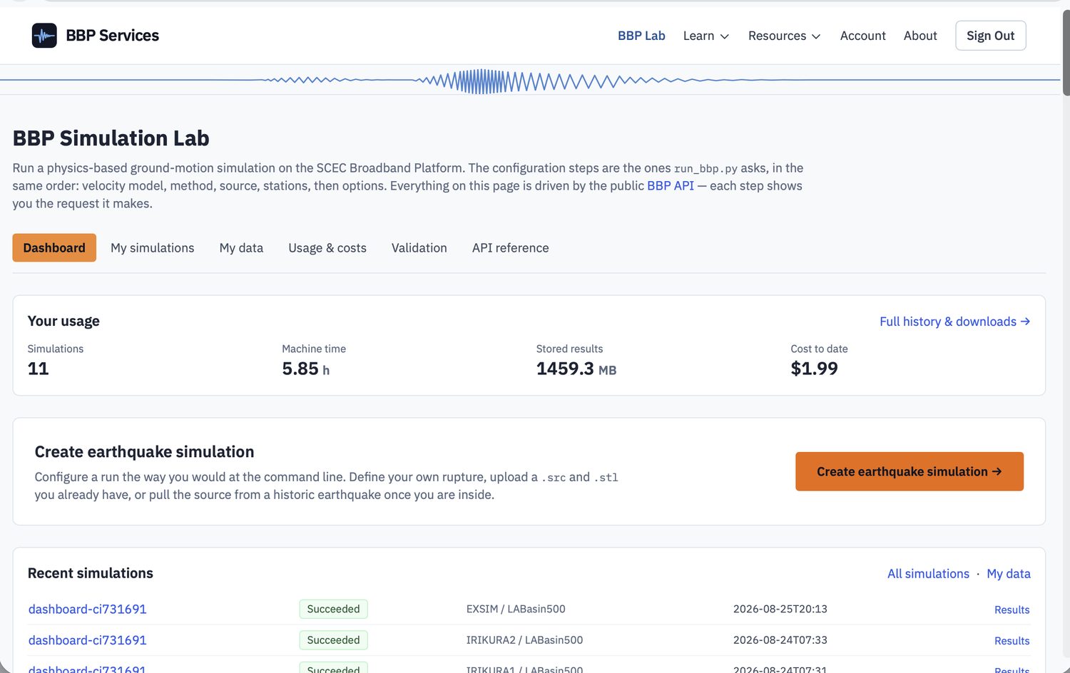
The dashboard opens on what your account has spent and what it is holding — simulations run, machine time, stored results, and cost to date — then the button that starts a new run, then the runs you already have. The tabs across the top are the whole Lab: the builder, your simulations, your stored data, usage and costs, the published validation results, and the API reference.

Usage is shown first on purpose. This is metered compute, and a page that made you go looking for the meter would be the wrong design.

The BBP Simulation Lab dashboard: a usage strip showing simulations, machine time, stored results and cost to date; a Create earthquake simulation button; and a table of recent simulations with their status, method and velocity model. — Usage, the way in, and recent runs. Each row names the method and velocity model it used, because those are what make two runs of the same earthquake different.

Building the job

Configuring a simulation

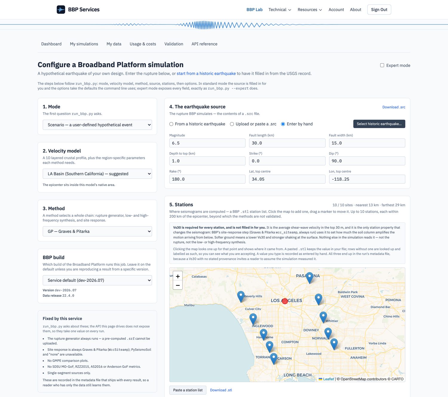
The builder is one page, numbered in the platform's own order. Pick a mode, a velocity model, and a method — a method is a whole chain, selecting the rupture generator, the low- and high-frequency synthesis and the site response together, so it is one choice rather than four. You also choose which build of the Broadband Platform runs the job, and the page prints the version it resolves to — together with the source repository and commit, where the build can attest to what it compiled. A version reported without a commit is a claim rather than a fact, so the page shows one only when there is one.

The source is the rupture itself — the contents of a .src file. Type it in, paste or upload one you already have, or start from a historic earthquake and have the geometry derived from the USGS record, then edit it. Standard mode fills in what the command line would default; expert mode exposes every field, including the hypocentre within the fault plane and the rupture seed.

A panel beside the form lists what this service fixes and does not let you change. Those choices are written into the metadata file that ships with every result, so someone who ends up with only the data still learns them.

The simulation builder: numbered panels for mode, velocity model, method and BBP build down the left; the earthquake source fields (magnitude, fault length and width, depth, strike, dip, rake, and the top-centre coordinates) at the upper right; and a station map below it with markers placed around Los Angeles. — The builder in standard mode, configuring a hypothetical M6.5 on a 30 km fault in the LA Basin, with ten recording sites placed across the basin. The panel on the left records which platform build will run it.

Stations, and the one value that is never guessed

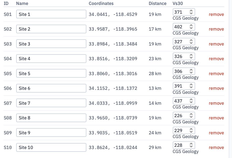
Stations are where seismograms get computed — a BBP .stl list. Click the map to add one, drag a marker to move it, or paste a list you already have. Each site has to be within 200 km of the epicentre, beyond which the methods are not validated.

Every station needs a Vs30, and the Lab will not silently supply one. It is the average shear-wave velocity in the top 30 m, and it is the only station property that changes the waveform — the site-response step uses it to set how much the soil column amplifies the motion arriving from below. Clicking the map looks a value up and shows you where it came from; a value you type is recorded as entered by hand. All three provenances end up in the run's metadata, because a Vs30 with no stated source invites a reader to assume the simulation measured it.

The station table: ten rows, each with an ID, an editable name, coordinates, the epicentral distance in kilometres, and an editable Vs30 value labelled with its source, CGS Geology. — Ten sites, each carrying its distance and a Vs30 labelled with where the number came from — here, CGS geology.

Before you commit

What it will cost

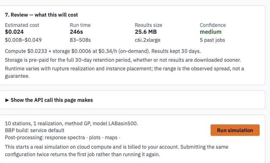
The last step of the builder is a quote. It updates as you change the configuration and gives you an estimated cost, an expected run time, how large the results will be, and how confident the estimate is — with the range and the number of past jobs the estimate is drawn from, so a first-of-its-kind run says so rather than pretending to precision it does not have.

Compute and storage are broken out separately, and storage is priced for the full retention period whether or not you download sooner. The quote and the eventual bill come from the same rate table on the server, so they cannot disagree.

The summary above the run button restates the job in one line — stations, realizations, method, model, build, post-processing — and tells you plainly that submitting starts a real run on cloud compute billed to your account. Submitting the same configuration twice returns the first job rather than running it again.

Getting the data out

Results

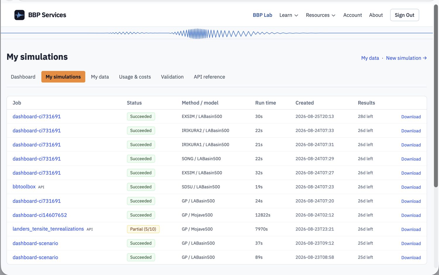
A submitted job appears in My simulations and updates as it runs. Each row carries its status, the method and velocity model, how long it took, and how much of its retention window is left. Jobs submitted directly to the API land in the same list as ones built in the Lab, marked as such — one account, one history, whichever way the job arrived.

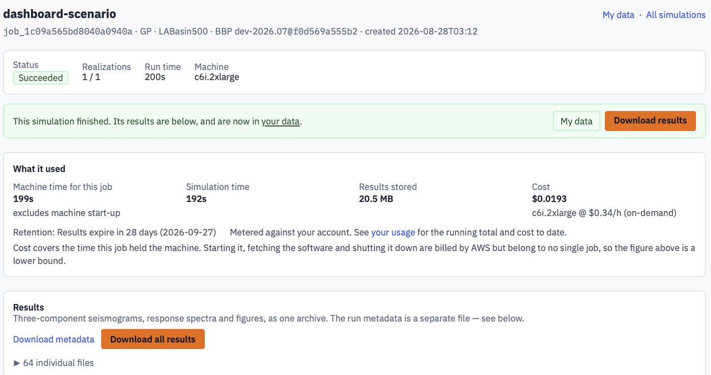
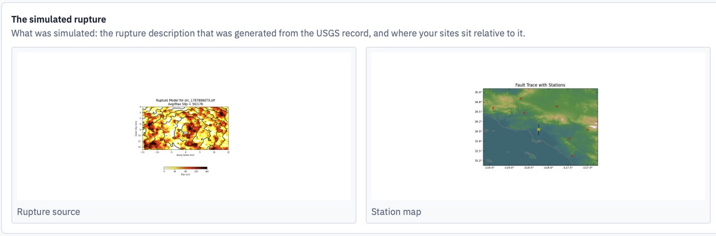
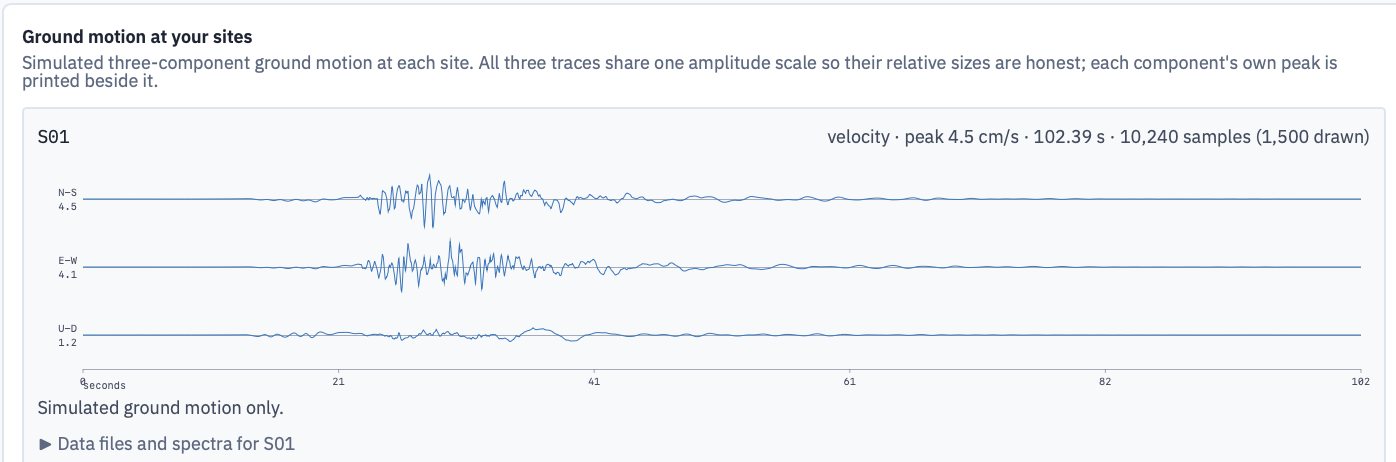
Opening a finished job gives you the results in the browser before you decide whether to download anything. The page leads with what the run used — machine time, simulation time, results size and cost — then the rupture that was simulated, then the ground motion at each of your sites, then the run metadata in full.

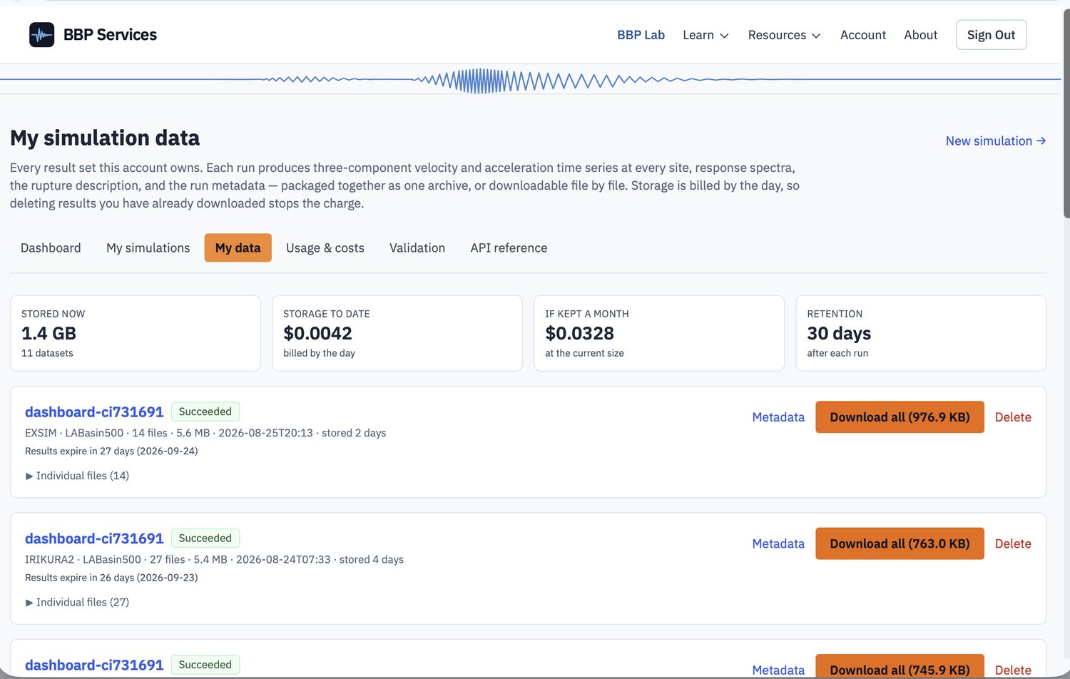
The files themselves are on My data. Every run produces three-component velocity and acceleration time series at every site, response spectra, the rupture description, and the run metadata — as one archive or file by file.

The top of a finished job's page: the job name with its id, method, velocity model, BBP build and creation time; a status strip reading Succeeded with realizations, run time and machine; a What it used panel giving machine time, simulation time, results stored and cost; and a Results panel offering the metadata and the full archive. — A finished run. The subtitle carries the method, the velocity model and the exact BBP build with its commit, so the page identifies what produced these seismograms rather than only when. *What it used* separates machine time from simulation time and says the cost is a lower bound — instance start-up and shutdown are billed by AWS but belong to no single job.

The simulated rupture panel of a finished job: two figures side by side, a rupture model coloured by slip across the fault plane, and a station map showing the fault trace with the recording sites marked around it. — What was actually simulated: the slip distribution the rupture generator produced, and where the sites sit relative to the fault. Not every method draws a rupture — a stochastic finite-fault method builds its fault from a parameter file and writes no rupture description, and the page says so rather than leaving an empty heading.

The ground motion panel for site S01: three stacked traces labelled N-S, E-W and U-D with their peak values, plotted against a 0 to 102 second time axis, headed 'velocity, peak 4.5 cm/s, 102.39 s, 10,240 samples (1,500 drawn)'. — One site's three components. They share a single amplitude scale so their relative sizes are honest, and each component's own peak is printed beside it. The header says how many samples were drawn of how many exist — the plot is decimated, keeping each bucket's extreme rather than a stride sample, so the peak you see is the peak in the data.

An expanded 'Data files and spectra for S01' panel: a Fourier amplitude spectrum thumbnail beside a list of four downloadable files - two response spectra files, a three-component acceleration time series and a three-component velocity time series - each with its size. — Each site expands to its own files: the Fourier amplitude spectrum, the response spectra, and the acceleration and velocity time series. You can take a single station's data without downloading the whole archive.

The My simulations table: one row per job with its name, a status badge, the method and velocity model, the run time in seconds, when it was created, how many days of retention remain, and a download link. — Every run this account has made. The rows marked API were submitted programmatically rather than built in the Lab.

The My simulation data page: tiles for stored bytes, storage billed to date, projected cost if kept a month, and the retention period; below them, one card per result set with its file count, size, expiry date, a Metadata link, a Download all button and a Delete link. — Stored results, with what each one is costing to keep. Storage is billed by the day, so deleting a result you have already downloaded stops the charge.

After the fact

Usage and costs

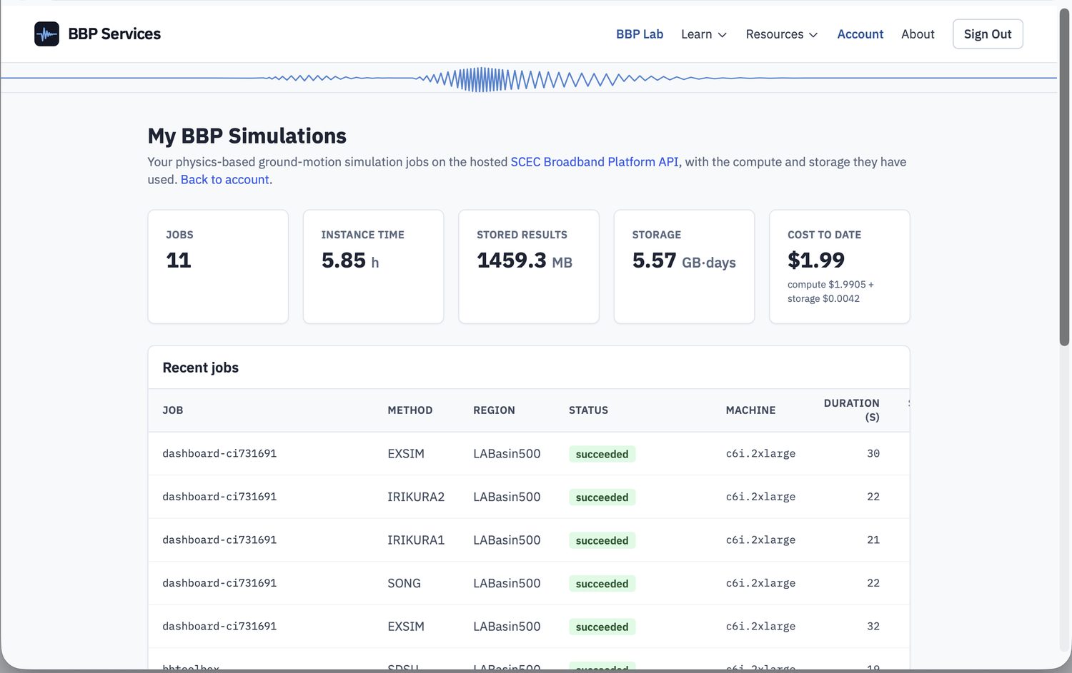
The Usage & costs tab opens the account's full meter — it lives on the account side, under the heading My BBP Simulations, because it covers everything the account has spent rather than only what the Lab submitted. Jobs run, instance time, bytes stored, storage in gigabyte-days, and cost to date split into compute and storage. Below it, every job is itemised with the machine it actually ran on and how long that machine was up.

The machine type is listed per job rather than assumed, because runs land on whatever instance capacity allows and the fleet is mixed. Cost is computed on the server from the same rate table the estimate quoted against, so what you were quoted and what you are billed are the same arithmetic on the same numbers.

The My BBP Simulations usage page: tiles for jobs, instance time, stored results, storage in gigabyte-days, and cost to date broken into compute and storage; below, a Recent jobs table listing each job's method, region, status, machine type and duration. — The meter for one test account. Every job names the machine it ran on and the seconds it was up — the two things the compute charge is computed from.

Checking the results are worth something

A simulated seismogram is only worth something if it resembles what a seismometer actually recorded. The Validation tab in the Lab, and the public verification and validation pages, publish that evidence: the curated SCEC validation events re-run against the recordings they ship with, and recent real earthquakes compared against data fetched from the seismic networks. Bias is reported period by period, not as a single average, because a simulation can look good on average and still be well off at the period a particular structure responds at.

See the verification & validation results →

Trying it yourself

Running a simulation costs money — it is metered compute, priced per job and billed to your account. Submitting is therefore enabled separately from registration: tell us what you want to run and we will turn it on. An account on its own gets you the Lab, the API reference and the published validation results. This is a prototype, and at this stage we are more interested in whether it is useful than in signing anyone up.

Create an Account → How the API works Or run the Broadband Platform yourself

The Broadband Platform is developed by the Statewide California Earthquake Center and its contributors and distributed under a BSD 3-Clause licence. BBP Services is an independent operator and is not affiliated with SCEC.